
This repo contains the files for the PCMLAI Module 11 Practical Assignment 2

In this application, you will explore a dataset from Kaggle. The original dataset contained information on 3 million used cars. The provided dataset contains information on 426K cars to ensure speed of processing. Your goal is to understand what factors make a car more or less expensive. As a result of your analysis, you should provide clear recommendations to your client -- a used car dealership -- as to what consumers value in a used car.
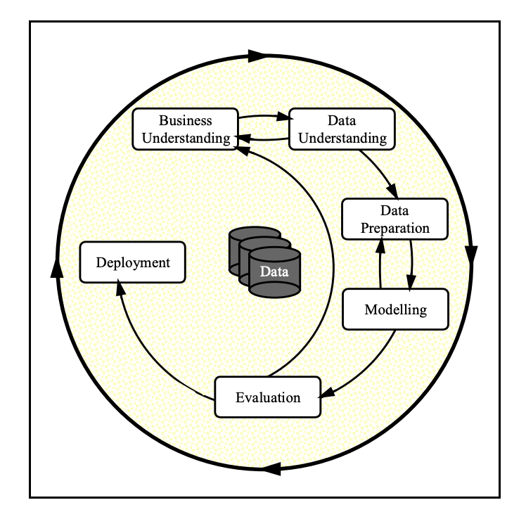
From a business perspective, we are tasked with identifying key drivers for used car prices. In the CRISP-DM overview, we are asked to convert this business framing to a data problem definition. Using a few sentences, reframe the task as a data task with the appropriate technical vocabulary.
-
Business Objectives: In order to run a successful used car dealership, the owner must price the used cars in a way that brings in profit. However, charging a high price for a used car is not the best way to sell used cars. The price must be reasonable enough to encourage customers to buy the used car from this dealership over other dealerships. The price must also be high enough to avoid losing profits. Determining what customers value in a used car and if those values can be used to accurately predict the price will allow the dealership to make a profit while gaining an advantage over competitors.
-
Assess the Situation: The business question will be answered using the vehicles dataset. This dataset contains information on over 400k used cars. It should be noted that this is a reduced version of the original dataset so a setback may be that the data isn't as accurate as it would be with more information. The data will be analyzed and used to create a model using Python and other libraries in a Jupyter Notebook.
-
Data Mining Goals: The intended output is a model that can predict the prices of used cars with as little error as possible on the validation set.
-
Project Plan: After cleaning the data, a multiple regression model must be created to predict the price of the used cars. To determine the features that will be used in the model, sequential feature selection will be used. While training the model, the dataset will be split into two sections, the training set and the validation set. The error of the model on the test set will be calculated using the mean squared error (MSE).
After considering the business understanding, we want to get familiar with our data. Write down some steps that you would take to get to know the dataset and identify any quality issues within. Take time to get to know the dataset and explore what information it contains and how this could be used to inform your business understanding.
- Collect the Data: Import the appropriate libraries and load in the dataset.
- Describe the Data: This dataset has 426k columns and 18 rows. These rows include attributes about the used cars. The features are id, region, price, year, manufacturer, model, condition, cylinders, fuel, odometer, title status, transmission, VIN, drive, size, type, paint color, and state.
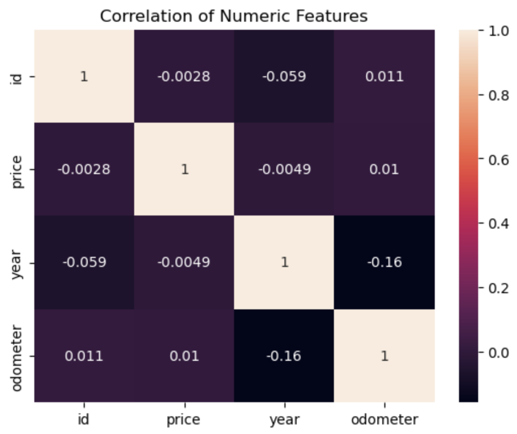
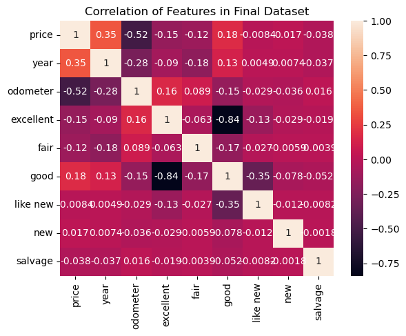
- Explore the Data: There are features that are likely to affect the price of a used car more than others. For example, the VIN number has no effect on the price of a car as it is only an identification number. The same can be said about the id column as it is simply just a way to identify the transaction for the car. Features like year, odometer, and condition are likely to have more of an effect on the price. A heatmap of the correlation between the numeric features (price, year, and odometer) shows that the odometer has more of a correlation to the price than the year does. This is because the odometer-to-price correlation is 0.01 and the year-to-price correlation is -0.0049. The odometer correlation is closer to 1 than the year correlation is to -1.
- Verify data quality: The data isn't very clean and will need data cleaning. There are a lot of missing data points that will need to be either deleted or filled with the column mode during data cleaning. There are also columns that can be deleted as they have no impact on the price of the car, like the VIN. There are also a few outliers, like significantly high prices and mileage, that must be dealt with.
After our initial exploration and fine-tuning of the business understanding, it is time to construct our final dataset prior to modeling. Here, we want to make sure to handle any integrity issues and cleaning, the engineering of new features, any transformations that we believe should happen (scaling, logarithms, normalization, etc.), and general preparation for modeling with sklearn.
Data Cleaning: Drop the "id", "model", "VIN", and "size" columns. The "id" and "VIN" columns have no effect on the price. The "model" column is filled with too many inconsistent values that may be a result of poor data collected like "ALL MAKES" and "2010 AND NEWER". Over half of the "size" column was filled with null values, specifically 71.77% of the column. Next, set the minimum and maximum values of the "price" and "odometer" columns to limit outliers based on industry knowledge. Then, fill in the remaining missing data with the mode of that column. Lastly, reset the index to end with a cleaner dataset.
With your (almost?) final dataset in hand, it is now time to build some models. Here, you should build a number of different regression models with the price as the target. In building your models, you should explore different parameters and be sure to cross-validate your findings.
I first reduced the dataset to include only the data that will be used during modeling (price, year, odometer, and condition (excellent, fair, good, like new, new, salvage)).
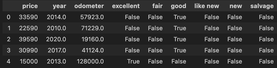
After splitting the data into two sets randomly, I created 5 different models.
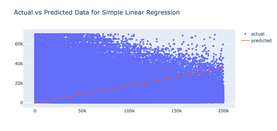
- Linear Regression Model: This model used the odometer feature to predict the price. However, for such a complex situation, using just one feature does not accurately predict price. Therefore, this model had a very high mean squared error (MSE) at 427469852.9022362. The one feature is not enough to predict the complex price as shown in this plot.
- Multiple Linear Regression Model With 2 Features: This model used the odometer and year features to predict price. This model did have less error compared to the linear regression model. However, it was not the best model. This model's MSE is 136340161.13806883.
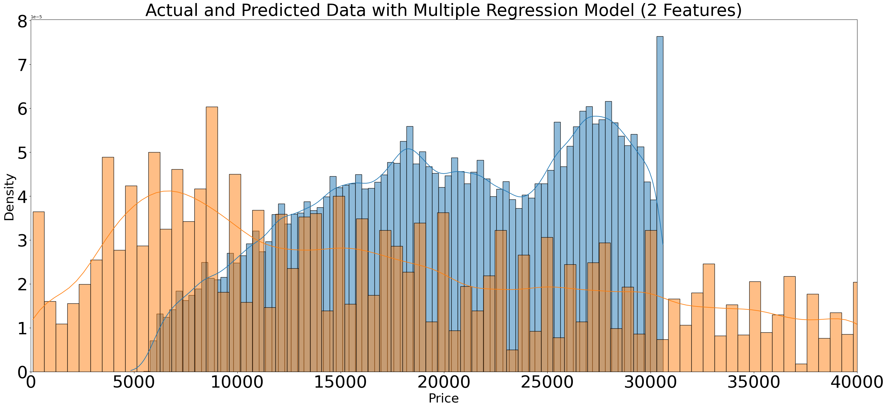
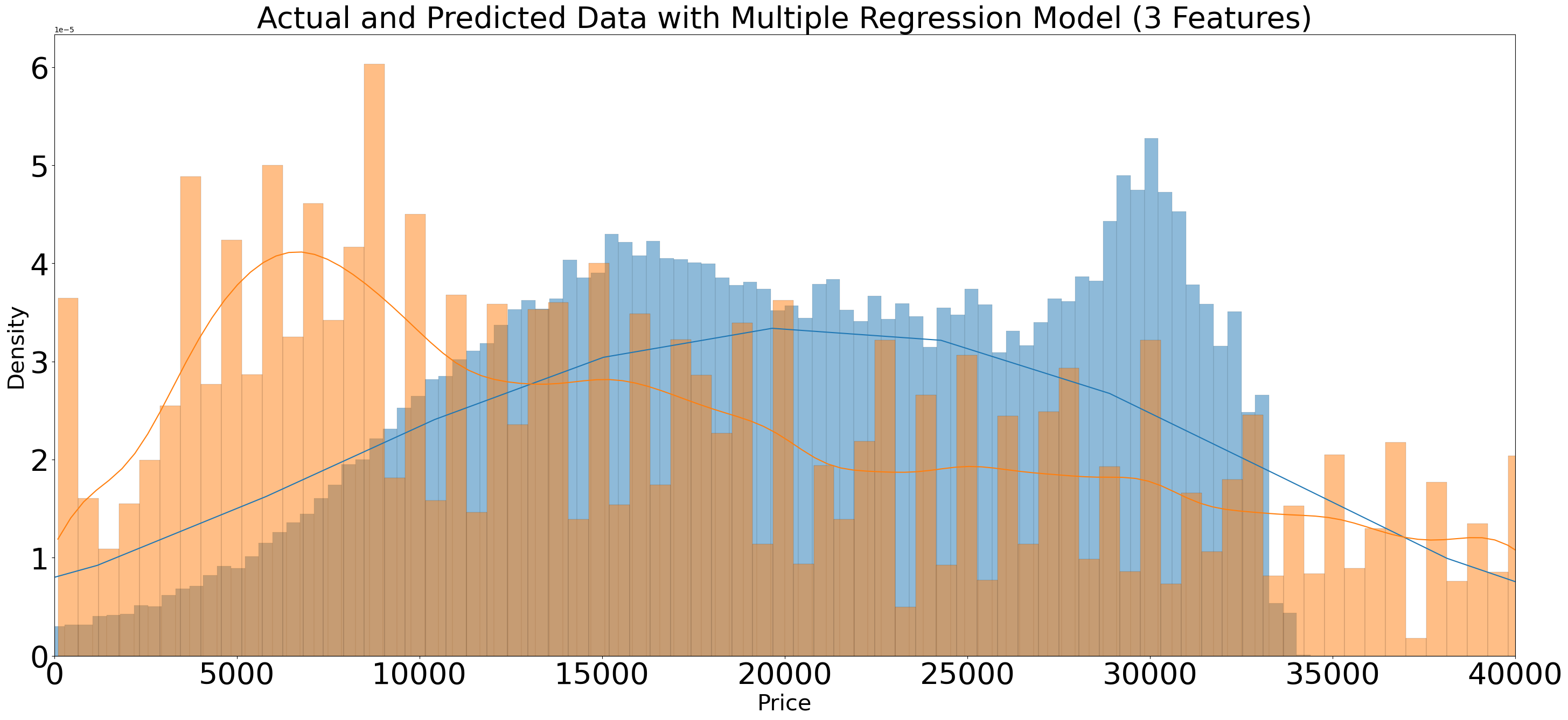
- Multiple Linear Regression Model With 3 Features: This model used the odometer, year, and condition features to predict price. It should be noted that the condition feature was deleted and expanded so that each value was given its own column. The MSE was at 10330032087.24176.
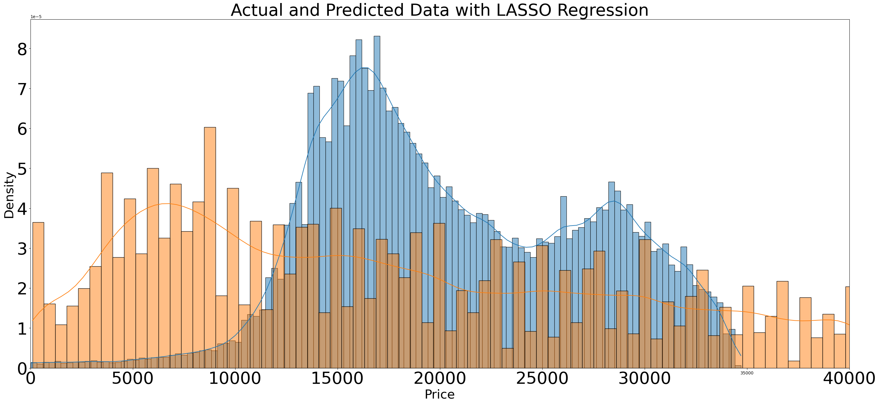
- LASSO Regression Model on Polynomial Features (Degree 2): This model used and squared the odometer and year features to degree 2 to predict price. This model did have less error compared to the linear regression model and multiple linear regression model with 2 features. However, it was not the best model. This model's MSE is 131124884.60776417
- Ridge Regression Model on Polynomial Features (Degree 3) Using GridSearchCV: This model used and cubed the odometer and year features to degree 2 to predict price. This was not the best model as this model only uses year and odometer to predict price. For a situation this complex, more features need to be included for better accuracy.
With some modeling accomplished, we aim to reflect on what we identify as a high-quality model and what we are able to learn from this. We should review our business objective and explore how well we can provide meaningful insight into drivers of used car prices. Your goal now is to distill your findings and determine whether the earlier phases need revisitation and adjustment or if you have information of value to bring back to your client.
Modeling was slightly difficult as performing hot encoding (creating numerical features for nonnumerical data) on all the nonnumerical features would have resulted in too large of a dataset to create models with. This meant that I had to choose a nonnumerical feature to turn into numerical data based on my industry knowledge. Nevertheless, various models were made, including a linear regression model, two multiple linear regression models, a LASSO regression model on polynomial features (degree 2), and a Ridge regression model on polynomial features (degree 3) using GridSearchCV.
The best model seems to be the multiple linear regression model with three features (year, odometer, and condition). This is because this model had the overall lowest MSE at 10330032087.24176. This model seems to have enough features to avoid overfitting (a model that memorizes and matches the data too closely) and underfitting (a model that does not match the data enough to preform well).
The linear model had a high MSE which makes sense as using one feature for such a complex situation falls victim to underfitting. It should be noted that the multiple linear regression model with two features had a better MSE but not as good as the one with three features. This is likely because numerical features are not the only factors that affect the price of a car. The LASSO regression (L1 Regularization) and Ridge Regression (L2 Regularization) models also did not do as well. This could be because these models were done solely on the numerical features which could have caused underfitting.
Features like the year, odometer, and condition of the car have an effect on the price of a car. These features should be used by the used car dealership to set prices that not only bring in profit but encourage customers to choose this dealership over others. The model can be used to predict accurate prices.
Additional information could be gathered. For starters, the original dataset should have fewer null data points. This way, the data will be more accurate and columns, like "size", will not have to be deleted. The data should also be collected carefully to avoid mistakes, like "ALL MAKES" in the "model" section. Further modeling could be done with other nonnumerical features, however, this will be more computationally expensive with hot encoding.
Now that we've settled on our models and findings, it is time to deliver the information to the client. You should organize your work as a basic report that details your primary findings. Keep in mind that your audience is a group of used car dealers interested in fine-tuning their inventory.
After extensively altering the data in a way that allowed for easier analysis and modeling, the best model was found. This model should predict the price based on the used car's year, odometer, and condition as they significantly affect the price of the used car. Based on the correlation to the price, the order of importance can be found. The odometer seems to be the most important with the price being the next in importance. When it comes down to the specific condition, customers seem to prefer a "good" used car over other conditions. Therefore, a used car with a high price should have fewer miles, be newer, and be in good condition. Although all the features in the dataset affect the price in some way (aside from the id and VIN), not all the features should be used when predicting price. Using the most important features allows accuracy and flexibility. Finding a good balance between numerical and nonnumerical features is important. So far, using the odometer, year, and condition features seems to be the "best" balance. For now, pricing can be predicted based on odometer, year, and condition. Variety in these features will result in varying prices. When it comes to inventory, the dealership should focus on buying cars that don't have too many miles, are fairly new (in terms of year), and are in good condition. Used cars that fall within this criterion are likely to be reasonably priced for customers and profitable for the dealership. These cars may even be able to be sold at slightly higher prices than predicted considering car prices are negotiable and this criterion is what customers look for most in a used car. Used cars that fall too far above or below this criterion may result in cars priced too low for the dealership to make a profit or too high for customers to afford. Accurate pricing is important as it encourages customers to choose this dealership over other dealerships; therefore, prices must be competitive yet profitable.
The next step would be to redo the data collection step. There are too many missing data points, outliers, and nonsensical data points for the model created to be the "best". There are also other factors that may affect the price of a car over the features mentioned in the dataset. One feature may be the time that the used car spent at the dealership as these cars may be cheaper. The time of year should also be considered as many dealerships have sales around the holidays. The price column also seems too vague. Car prices are negotiable and tend to rise and fall depending on the buyer and salesman. The price can be split into sales price and transaction price.
If the dealership owner wishes to use the dataset as is and avoid further data collection. The next step would be using the current model (multiple linear regression model with 3 features) to predict the prices of the used cars in the dealership currently. It may be beneficial to do further modeling. This can be done with other nonnumerical features like region, fuel, or cylinders. Considering further modeling with nonnumerical features requires the nonnumerical values to be turned into numerical columns, this process would be tedious as turning all of the nonnumerical features into numerical ones is too much for most computers considering the current dataset is already pretty large. Other ways of making the nonnumerical values numerical may be more beneficial as the current method is computationally expensive. Nonetheless, it is beneficial to the used car dealership, in the long run, to find the perfect balance of numerical and nonnumerical features for predicting the price after better data collection and cleaning.
The link to the Jupyter Notebook with the coding for this project can be found here. It should be noted that the vehicles dataset and the file with the coding for this project are both too large to automatically display in GitHub. Both files must be downloaded in order to view them. The file with the coding specifically must be downloaded in Visual Studio Code and the workspace must be trusted in order to completely view the coding and plots.